Wasserstein NMF on histograms representation of mixtures of gaussians

This script is intended as a usage example of the Wasserstein Dictionary Toolbox, it reproduces the experiment in the introduction of [paper]

Contents

Generate the data

ndata=100;              % number of mixtures
niidsample=1000;        % number of sample for each mixture
ndiscretize=100;        % number of histogram bins

minVal=-12;
maxVal=12;
x=linspace(minVal,maxVal,ndiscretize);  % value of the histograms bins

mu=[-6;0;6];                            % mean values for the Gaussians means
shiftVariance=2*eye(3);                 % variance of the Gaussians means
mean=mvnrnd(mu,shiftVariance,ndata)';   % generate the gaussian means
p=rand(3,ndata);                        % generate the mixture weights

sigma=1;                                % variance of the Gaussians

data=zeros(ndiscretize,ndata);          % preallocate memory
for i=1:ndata
    distrib=gmdistribution(mean(:,i),sigma,p(:,i)); % generate a mixture of gaussians distribution
    a=random(distrib,niidsample);                   % sample the distribution
    data(:,i)=hist(a(a>minVal&a<maxVal),x)';        % gather samples in a histogram
end

data=bsxfun(@rdivide,data,sum(data));   % normalize the data

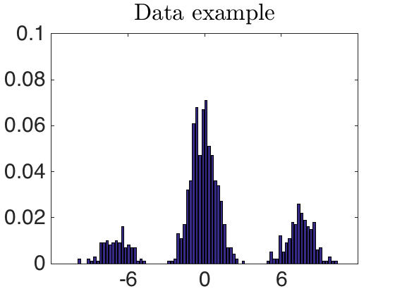
Visualize the data

minY=0;
maxY=.1;
YtickStep=.02;
i=1;
fontSize=30;
lineWidth=3;


bar(x,data(:,i))
set(gca,'FontSize',fontSize)
axis([minVal, maxVal, minY, maxY])
set(gca,'yTick',minY:YtickStep:maxY)
set(gca,'xTick',mu)
set(gca,'defaulttextinterpreter','latex');
title('Data example')

Build the cost matrix

M=abs(bsxfun(@minus,x',x));
M=M/median(M(:));

Set the parameters of wasserstein_DL

options.stop=1e-3;
options.verbose=0;
options.alpha=0.5;
options.Kmultiplication='symmetric';
options.GPU=0;
k=3;

gamma=1/50;

wassersteinOrder=1;

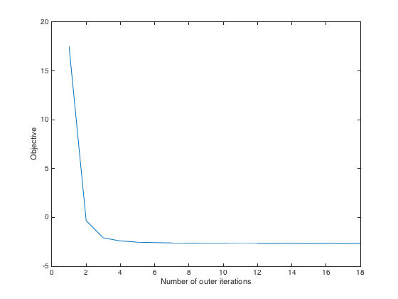
Perform Wasserstein DL

options.alpha=0.5;
options.D_step_stop=1e-7;
options.lambda_step_stop=1e-7;
tic;
[D_DL, lambda_DL, objectives]=wasserstein_DL(data,k,M.^wassersteinOrder,gamma,0,0,options);
toc
plot(objectives);
xlabel('Number of outer iterations')
ylabel('Objective')

Elapsed time is 5.045597 seconds.

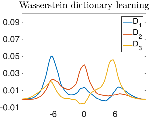
Visualize the dictionary

minY=floor(min(D_DL(:)*100))/100;


plot(x,bsxfun(@rdivide,D_DL,sum(abs(D_DL))),'LineWidth',lineWidth)
set(gca,'FontSize',fontSize)
axis([minVal, maxVal, minY, maxY])
set(gca,'yTick',minY:YtickStep:maxY)
set(gca,'xTick',mu)
set(gca,'defaulttextinterpreter','latex');
legend('D_1','D_2','D_3');
title('Wasserstein dictionary learning')

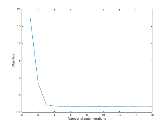
Perform Wasserstein NMF

rho1=.1;
rho2=.1;
options.D_step_stop=5e-5;
options.lambda_step_stop=5e-4;
tic;
[D, lambda, objectives]=wasserstein_DL(data,k,M.^wassersteinOrder,gamma,rho1,rho2,options);
toc
plot(objectives);
xlabel('Number of outer iterations')
ylabel('Objective')

Elapsed time is 29.500731 seconds.

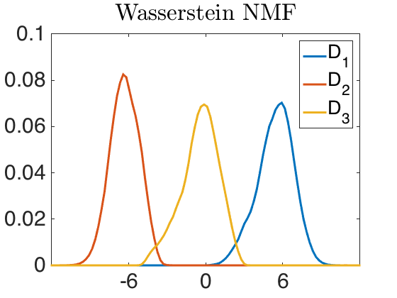
Visualize the dictionary

minY=0;
plot(x,bsxfun(@rdivide,D,sum(abs(D))),'LineWidth',lineWidth)
set(gca,'FontSize',fontSize)
axis([minVal, maxVal, minY, maxY])
set(gca,'yTick',minY:YtickStep:maxY)
set(gca,'xTick',mu)
set(gca,'defaulttextinterpreter','latex');
legend('D_1','D_2','D_3');
title('Wasserstein NMF')

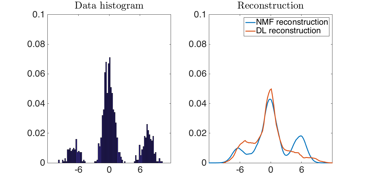
Compare data and reconstruction

width=1200;
height=600;
figure('Position',[1 1 width height])

minY=0;
i=1;

subplot(1,2,1)
bar(x,data(:,i))
set(gca,'FontSize',3)
set(gca,'FontSize',30)
axis([minVal, maxVal, minY, maxY])
set(gca,'yTick',minY:YtickStep:maxY)
set(gca,'xTick',mu)
set(gca,'defaulttextinterpreter','latex');
title('Data histogram')


subplot(1,2,2)
plot(x,[D*lambda(:,i),D_DL*lambda_DL(:,i)],'LineWidth',lineWidth)
set(gca,'FontSize',fontSize)
axis([minVal, maxVal, minY, maxY])
set(gca,'yTick',minY:YtickStep:maxY)
set(gca,'xTick',mu)
set(gca,'defaulttextinterpreter','latex');
legend('NMF reconstruction','DL reconstruction')
title('Reconstruction')

Published with MATLAB® R2015a